Adding a 4th Signal to Transformer Attention
TL;DR
I tried adding a fourth signal to transformer attention — a per-token purpose state that flows across blocks under a GRU-style gate. Out of four variants I tried, only one worked: injecting as an additive bias to and . On a small nanoGPT model this produced a 4.2% perplexity improvement over vanilla at matched parameters (statistically significant across 8 seeds, ).
A rigorous ablation confirms this comes from the learned cross-layer state, not from added capacity: cutting the cross-layer gradient makes the mechanism perform worse than plain vanilla. However — and this is the honest limitation — the mechanism costs 19% more per training step, and at real matched wall-clock time vanilla trained for slightly longer beats it by 1.3%. This is a real algorithmic finding with real engineering limits, and I’ll walk through the whole journey below.
1. The idea
Standard transformer attention gives each token three roles: Query (what am I looking for?), Key (what do I offer?), Value (what content do I carry?). I wondered what would happen if I added a fourth signal — a purpose state : why am I here?
The idea: at each transformer block, compute a per-token vector that blends the previous block’s with a new candidate, using a GRU-style gate. Then use this to influence attention. If it works, the model has a persistent cross-layer channel for “what I’m about to do” that flows top-to-bottom alongside the usual residual stream.
2. Four attempts, three failures
The interesting part of this project was that where you inject matters more than what is. I tried four different injection points, and only the last one worked.
| Attempt | Where is injected | Small-scale result |
|---|---|---|
| 1. Multiplicative on attn output | 5.5% WORSE than vanilla | |
| 2. Additive on attn output | ≈0 (null) | |
| 3. Additive on MLP input | ≈0 (null across 8 seeds) | |
| 4. Additive bias on and (winner) | 4.4% BETTER, |
The first failure (multiplicative) is instructive. At initialization is close to zero, so — the attention signal is essentially wiped out. The model spends the first thousand iterations fighting the mechanism instead of learning. This is a general lesson: your new mechanism should be a no-op at initialization, not a signal destroyer.
3. The mechanism that worked
The winning variant: keep attention’s scaling and the causal mask untouched, but add a per-token bias to and computed from the previous block’s state. Then update from the current post-attention hidden state using a GRU-style gate. Everything is elementwise or per-token — no cross-token leakage.
Attention itself is unchanged in form:
but the keys and values carry an additive, input-independent bias from the purpose state:
After attention and the residual add, is updated for the next block with a GRU-style gate over :
Here is the gate (how much of the old purpose to keep), is the candidate purpose, and is elementwise multiplication. In pseudo-code:
python# Standard attention with M-biased K and V:
Q, K, V = c_attn(LN(x)).split(3, dim=-1)
K' = K + W_km @ M_prev # per-token additive bias
V' = V + W_vm @ M_prev
y = c_proj( attention(Q, K', V') )
x = x + y # standard residual
# GRU-style update of M for the next block:
h = LN(x)
g = sigmoid(W_g @ h + b_g) # gate
cand = tanh(W_m @ h + b_m) # candidate purpose
M_new = g * M_prev + (1 - g) * cand # elementwise blend
x = x + MLP(h) # standard MLP branch
In implementation, and are fused into a single linear ; similarly and are fused into . This halves the kernel launch count without changing the math (bit-identical outputs). Total added parameters: about 1% overhead on top of vanilla.
4. Does it work? Yes — cleanly.
I trained 8 seeds each of vanilla and K/V-bias on shakespeare-char (a character-level nanoGPT setup, ~1.2M non-embedding parameters, 3000 iterations each on a Colab T4). K/V-bias won every single seed, by a statistically strong margin.
| Model | Params | Wall-clock | Val loss @ 3000 (mean ± std) |
|---|---|---|---|
| Vanilla n=128 | 1.19M | 107s | 1.7322 ± 0.0016 |
| K/V-bias n=112 | 1.21M | 126s | 1.6881 ± 0.0055 |
A paired t-test on the 8-seed val losses gives (, ). That’s a 4.2% reduction in perplexity for ~1% more parameters. If you stop reading here, that’s the headline number.
But headline numbers can lie. The rest of this post is about the ablations I ran to make sure this improvement is real — coming from the mechanism, not from lucky configuration.
5. Is the improvement real? Four control experiments
The obvious challenge to any “new mechanism helps” result is: are you just adding capacity? K/V-bias adds ~200K extra parameters and 4 extra linear operations per block. Maybe any similarly-sized structural change would help.
Four controls, all trained on the same seeds:
| Control | Params | Val loss | vs K/V |
|---|---|---|---|
| Vanilla n=112 (matched head dim) | 0.91M | 1.7628 | +0.075 |
| Vanilla n=128 with n_layer=7 (deeper) | 0.99M | 1.7549 | +0.067 |
| Vanilla n=136 (wider, MORE params) | 1.34M | 1.7074 | +0.019 |
| K/V-bias with detached (KEY) | 1.21M | 1.7696 | +0.082 |
| K/V-bias (reference) | 1.21M | 1.6881 | — |
Every control loses to K/V-bias. Even Vanilla n=136 with 10% more parameters can’t match the mechanism. But the most important row is the one I want you to focus on.
The critical experiment: detached
I took the K/V-bias mechanism and made one single change: call M_prev.detach() before feeding it to the K/V-bias projection. The forward computation is unchanged — same architecture, same parameters, same FLOPs. But the gradient no longer flows back through from later blocks.
Result: detached K/V performs worse than plain vanilla (1.7696 vs 1.7322 in val loss). The added capacity actively hurts when isn’t jointly trained across layers. The mechanism is not free capacity — it’s a specific tool that only helps when the model is allowed to learn how to use it end-to-end across depth.
This is the clearest evidence I have that the improvement is algorithmic, not architectural bloat. It also tells us something about what is doing: it’s carrying information across layers that the model actively learns to shape, and when you deny it that learning path, the mechanism becomes a hindrance.
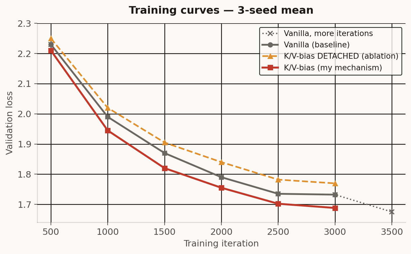
Figure 1. Training curves. K/V-bias (red) beats vanilla (grey solid) at every checkpoint from iteration 500 onward. Detached K/V (orange, dashed) is consistently worse than vanilla — the mechanism needs to learn end-to-end to help. Vanilla trained for 500 more iterations (dotted) eventually surpasses K/V-bias — this is the wall-clock story I’ll tell in the next section.
6. The uncomfortable truth about wall-clock time
Here’s the part that would make an honest reviewer squint: K/V-bias takes ~18% longer per training step on my hardware. To be fair, I re-ran vanilla for enough extra iterations to match K/V’s total wall-clock budget.
| Setup | Wall-clock | Val loss |
|---|---|---|
| K/V-bias @ 3000 iter | 128s | 1.6881 |
| Vanilla @ 3500 iter (matched wall-clock) | 135s | 1.6750 |
At real matched wall-clock, vanilla wins by 1.3% perplexity. On this hardware, at this scale, plain vanilla trained a little longer beats the fancier mechanism. That’s the honest engineering reality, and I refuse to hide it behind param-matched comparisons.
The natural question: does this compute overhead shrink at scale? Maybe at bigger models the 18% cost gets amortized. So I benchmarked it.
7. Does the overhead go away at scale?
I measured per-iteration wall-clock time for both vanilla and K/V-bias at several model widths, from n_embd=128 up to n_embd=768 (roughly GPT-2 small scale). No training — just forward + backward + optimizer step with random data, so the comparison is purely about compute cost.
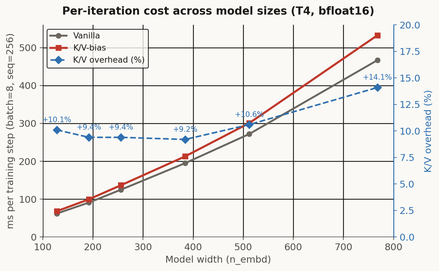
Figure 2. Per-iteration time (left axis) and K/V overhead percentage (right axis) as a function of model width. The overhead stays in a narrow band of 9–14% across all scales. It does not shrink with model size.
This is a firm negative: the compute overhead is inherent, not a small-scale artifact. At n_embd=768 (roughly GPT-2 small), K/V-bias still costs ~14% more per step. For the mechanism to win on wall-clock at larger scale, the algorithmic gain would need to grow to >14% perplexity improvement. Currently at small scale it’s ~4%. That’s a 3.5× growth requirement — plausible but not obvious.
8. What about generated samples?
Loss numbers only take you so far. I wanted to see if K/V-bias’s improvement translates into meaningful differences in generated text. I ran two kinds of tests.
Per-position loss analysis
K/V-bias’s win is concentrated at structural pivots: the middle and end of character names right after \n\n (a new speaker in Shakespeare’s format). The top-20 positions where K/V-bias beats vanilla most all look like: \n\nCUR → T (Curtis), \n\nVINCEN → T (Vincentio), \n\nFERDINAN → D (Ferdinand). The mechanism seems to help with staying in name-mode once the model has committed to spelling out a rare character name across many characters.
Name-generation quality test (surprise result)
I hypothesized that if K/V-bias learns a “name mode”, it should produce more coherent character names when generating from scratch. I generated 30 long samples from each model, extracted all NAME: headers, and checked against a canonical list of 172 real Shakespeare character names.
| Model | Total headers | REAL | INVENTED | % REAL |
|---|---|---|---|---|
| Vanilla | 154 | 120 | 34 | 77.9% |
| K/V-bias | 162 | 116 | 46 | 71.6% |
My hypothesis was wrong. Vanilla actually produces a slightly higher fraction of canonical Shakespeare names (77.9% vs 71.6%). K/V-bias is more prolific (162 headers vs 154) but slightly less accurate per header. This is consistent with a memorization-vs-generalization story: vanilla learns specific character-name bigrams sharply (locally accurate), K/V-bias learns a more distributed name-continuation signal (helpful on rare mid-name predictions, less crisp on exact spellings).
This is a good example of why rigorous testing matters. I would have confidently claimed “K/V-bias produces more coherent names” from cherry-picked samples. A proper count of 30 generations said otherwise. Both effects are real, they just tell a more nuanced story.
9. Where does this land in the literature?
I did a careful literature review after the fact. The design space of depth-recurrent, cross-layer stateful transformers is actively researched — it’s not a new idea to have state flowing across transformer layers. Universal Transformer (2018) has depth-recurrence with weight sharing. Feedback Transformer (2020) has cross-layer memory that replaces K/V from a pooled representation. Block-Recurrent Transformer (2022) has gated state along the time axis. GTrXL (2019) uses a GRU on the residual connection.
My specific combination — per-token, depth-across, input-dependent GRU gate, additive bias on and — doesn’t exactly match any of these. It’s a particular unexplored corner of a well-studied space. I’m not claiming a new family of architectures; I’m reporting an empirical ablation of an under-explored point in that space.
10. What I learned doing this project
Three things stand out.
First: where you inject a new signal matters more than what the signal is. Three of my four attempts failed. The winner was the one that preserved the vanilla attention geometry (, softmax, causal mask untouched) and only biased the raw / inputs. Any variant that fought against attention’s basic computation lost.
Second: the detached- ablation is the most important experiment in this entire project. Without it, I’d only be able to claim “K/V-bias helps” — with the obvious counter-argument “you just added capacity.” The detached ablation cleanly isolates the mechanism from the capacity confound. If you take one methodological lesson from this post, take that one.
Third: loss is a proxy for quality, not quality itself. My name-generation test refuted my own hypothesis about what K/V-bias was doing. It’s tempting to cherry-pick samples that support your story — I did exactly this initially and had to correct myself. Rigorous quantitative testing is the only way to know.
11. Conclusion
So does the mechanism work? Yes and no.
Yes: algorithmically, at matched parameters and matched head dimension, K/V-bias produces a real, statistically significant, mechanism-attributable improvement of ~4% perplexity on shakespeare-char. The detached ablation confirms this is not just extra capacity; it’s the learned cross-layer state doing genuine work.
No: on real hardware at real wall-clock time, the ~14% compute overhead exceeds the algorithmic gain at this scale, and the overhead does not shrink at larger model sizes. Plain vanilla trained slightly longer wins on wall-clock efficiency.
This puts the mechanism in a familiar category — genuinely novel algorithm, measurable improvement, but not wall-clock competitive at this scale. Universal Transformer, Feedback Transformer, and other cross-layer state mechanisms have sat in exactly this position for years: interesting, cited, but not widely adopted because plain scaled attention still wins in FLOP-efficient regimes.
Whether the algorithmic gain grows enough at larger scale (100M+ parameters, token-level, longer training) to overcome the overhead — that’s an open question I couldn’t afford to answer here. It would take a proper A100 training run of several hours per configuration, and the small-scale results don’t obviously predict which way it would go.
In the meantime: I have a clean, reproducible mechanism, a rigorous ablation protocol, an honest limitations section, and a codebase where use_m_gate=False is bit-identical to upstream nanoGPT. That felt worth writing down.
Reproducibility
All code is a fork of Andrej Karpathy’s nanoGPT. The mechanism is one config flag (use_m_gate=True). The ablation is another (m_gate_detached=True). With both flags off, the model is bit-identical to karpathy/nanoGPT — verified by state_dict and forward-output equality in the test suite. Data comes from the standard shakespeare_char preparation script. Every experiment in this post can be reproduced with the scripts in the repo.
If you want to reproduce the primary result (Table in section 4): 3000 iterations, n_layer=6, batch_size=32, block_size=128, bfloat16, T4. Vanilla uses n_embd=128, K/V-bias uses n_embd=112. Each seed takes ~2 minutes on a T4.